Extraction Coefficients

In this page you will find an explanation about what extraction coefficients are, how they can be used to define function spaces, and how they can be used in Mantis.

Recommended Reading

Before reading this page it's advised that you have a basic understanding of The Finite Element Method (FEM). That way, you can fully appreciate why the ideas discussed here are useful.

Introduction

One of the fundamental ideas in FEM is that you discretise a continuous problem, converting it into a finite-dimensional algebraic system you can solve numerically. For our purposes, you can think of taking a PDE and turning it into a linear system of equations. There are usually two distinct but interconnected layers to the discretisation:

• A computational mesh, composed of elements, that represents the domain of the continuous problem.

• One or more finite-dimensional function spaces defined on the computational mesh.

A fruitful way to think about the function spaces is in terms of their degrees of freedom. In essence, because we deal with finite-dimensional function spaces, we can find a similarly finite-dimensional basis whose basis functions can be combined to represent any function in the function space. A simple example is representing a linear function   . A basis for the space of linear functions is of course . Therefore, if we choose a coefficient vector  , we get

But there is no real reason to stick with — other than it being a natural choice. We could have also chosen as a basis   , which of course means the coefficient vector will have to be different if we still want to represent ; in this case, it would be  . With this we get

The key takeaway is that given a basis  , we can use a coefficient vector   to represent any function in the span of by  .

Classical FEM

In classical FEM, the connection between the mesh and the function spaces is quite pronounced. It's almost always the case that degrees of freedom will be tied to some component of the mesh. For instance, we might associate some degrees of freedom to the vertices, and others to the edges, or faces. This is in general quite a profound idea, with important consequences for solving PDE arising from physics problems. For example, solving for a temperature is meaningful at points, or vertices, while solving for a density makes more sense when using volumes. The details are beyond the scope of this page, but it is something interesting to keep in mind.

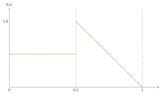
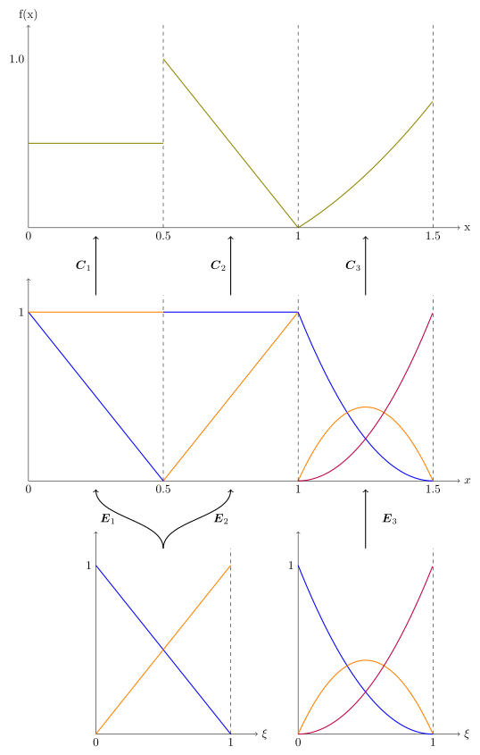
Still in the spirit of classical FEM, we can extend the previous example to piecewise-linear functions over a given mesh; meaning that restricted to an element of the mesh, any function is linear. We will consider a simple one-dimensional mesh composed of two elements: and ; we label them as and . For the function, we will define such that   and   . Below is what looks like.

The difference from what we saw in the beginning of the introduction is that in each element we will have a local basis. This basis works the same way as the global example we saw before, but because our function is piecewise-linear it only makes sense to use a basis for linear functions restricted to a given element. So, we have

where denote the local basis at element , and the coefficient vector that pertains to the basis functions supported on element . We can visualise it as follows:

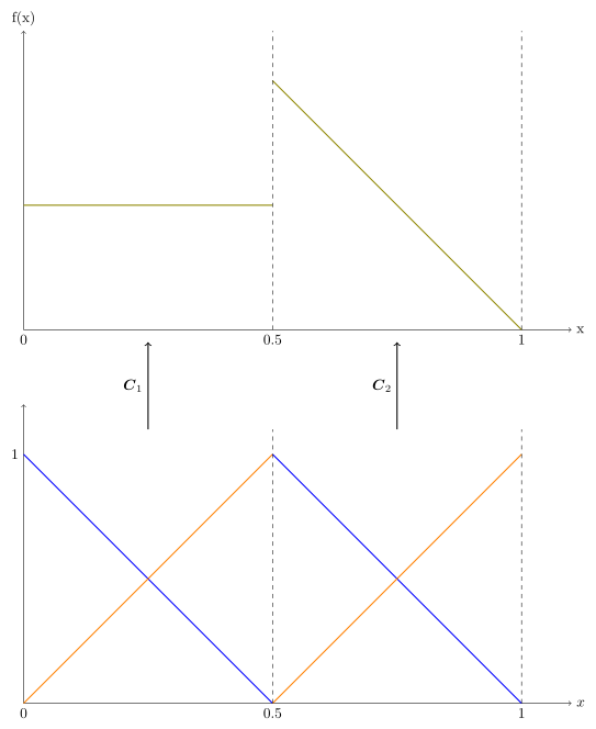
You might have noticed that the local bases in each element are identical. Therefore, these bases can be described in terms of a single basis for linear functions, that is then linearly combined to define a new local basis in each element. We write it as such:

where is a canonical basis, or section space, that is independent of the element , and are the extraction coefficients saying how the canonical basis is linearly combined to form a local basis at element . Here is what it looks like for our example:

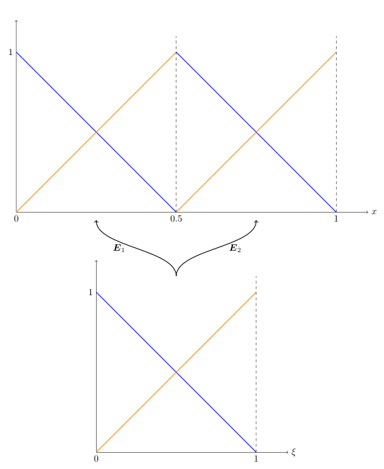
This in turn means that we can write

Putting it all together we get:

A note on efficiency

This might seem overly complicated at first, but it is very valuable from a computational perspective. By using extraction coefficients, the canonical basis can be computed once, and later referenced to define the local basis on each element. This means that we replace computing the “same” basis on each element with matrix multiplications, which is in general much cheaper.

Generalisation

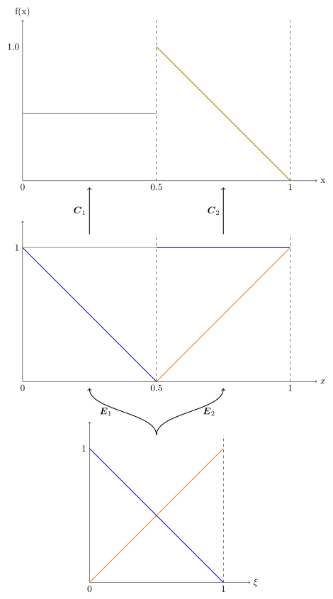
In the last figures we saw that the two local bases looked identical. This does not need to be the case. The local basis can be different across elements. This is also a powerful realisation. By using this framework, we can use the same canonical basis to define completely different local bases. As we will see later using Mantis, this makes it possible to change the inter-element smoothness of our global basis without changing the canonical basis.

Finally, we can generalise this even further. We might want multiple canonical basis, which are then linearly combined to define local bases in whatever combination we choose. Below is an example of what this might look like if we extend our example so that is quadratic over a new element

Implementation in Mantis

Note

The details that follow are low-level in the Mantis framework. The only real reason you would have to use ExtractionOperator directly is when implementing your own function space. Even then, it is very unlikely that you will be tweaking each matrix manually as will be done below. The following examples serve only to showcase what information the structure encodes.

In Mantis, all the information pertaining to the extraction-coefficient framework is implemented in two structures:

• Indices

• ExtractionOperator

We will now consider a more general case than in the Introduction: multi-component function spaces. Another common name for these types of spaces is vector fields.

An example of a multi-component space

A simple example is a direct-sum space in two dimensions: Given two function spaces     , we can define the direct-sum space     by

Then given   , we have  .

Indices

On a given element, not all global basis functions are supported — only those whose support has a non-empty intersection with the element. The Indices struct tracks which global basis functions are active on an element, and in what order they appear when the canonical basis is evaluated. Concretely, it stores:

• I: a vector of global indices identifying the basis functions that are supported on the element. This is used to assemble element contributions into the global system.

• J: an NTuple with one entry per component of the space. Each entry is a permutation that encodes how the local basis functions are arranged into the global bases at a given element and component.

Permutation J

The permutation operator J is useful when defining multi-component spaces that can not be written as direct-sum spaces. In these cases, it is necessary to define how the local bases from a given component contribute to the global, multi-component basis — possibly contributing to multiple components.

You can find the full details at FunctionSpaces.Indices.

ExtractionOperator

The ExtractionOperator aggregates all element-level data for a function space:

• extraction_coefficients: a length-num_elements vector. Each entry is an NTuple{num_components} of matrices: one matrix per component . The matrix encodes how a canonical basis is linearly combined to form the local basis on element for component :

  Remember: It is possible that a permutation with J occurs.

• basis_indices: a length-num_elements vector of Indices objects, one per element.

• num_elements: the total number of elements.

• num_basis: the global dimension of the function space — or number of degrees of freedom.

You can find the full details at FunctionSpaces.ExtractionOperator.

Interface

To avoid having to directly access fields of ExtractionOperator, Mantis provides a small set of “getters”:

Method	Returns
FunctionSpaces.get_extraction(space, element_id, component_id)	(E_e, J) — the extraction coefficient matrix and permutation indices for element element_id and component component_id
FunctionSpaces.get_extraction_coefficients(space, element_id, component_id)
FunctionSpaces.get_basis_indices(space, element_id)	global index vector I for that element
FunctionSpaces.get_basis_permutation(space, element_id, component_id)	local permutation J for that element and component
FunctionSpaces.get_num_basis(space)	total number of degrees of freedom
FunctionSpaces.get_num_basis(space, element_id)	number of basis functions supported on an element

Putting it together

To evaluate the global basis on element element_id at a set of points xi, Mantis executes the following steps (see FunctionSpaces.evaluate for the details):

• Get support indices: I = get_basis_indices(space, element_id) identifies the columns of the global evaluation matrix that this element contributes to.

• Loop over components: For each component :

  • Retrieve the stored   .

  • Evaluate the canonical basis on the reference element.

  • Compute the local basis evaluations via the matrix product  .

  • Place the result into the columns selected by .

• Return: The evaluated global bases with the global support indices I.

This design keeps the canonical-basis evaluations element-agnostic (they are computed once on a canonical domain) while all element-specific information is encoded in the ExtractionOperator data structure.

Example: inspecting the extraction operator

We will use as canonical basis the quadratic Bernstein polynomials.

bern = FunctionSpaces.Bernstein(2)
xi = LinRange(0, 1, 50)
points = Points.PointSet(xi)
bern_eval = FunctionSpaces.evaluate(bern, points, 0)[1][1]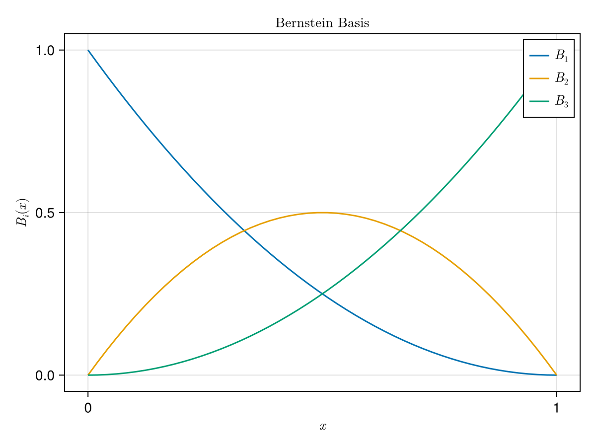

We can then use this canonical basis to create a BSplineSpace on a 5-element geometry, by specifying the inter-element regularity.

const geo = Geometry.create_cartesian_box((0.0,), (1.0,), (5,))
bsp = FunctionSpaces.BSplineSpace(geo, bern, [-1, 0, 1, -1, 1, -1])

The inter-element regularity vector [-1, 0, 1, -1, 1, -1] is specifying how smooth the B-Spline space is across element interfaces. With our choice, our functions will be: 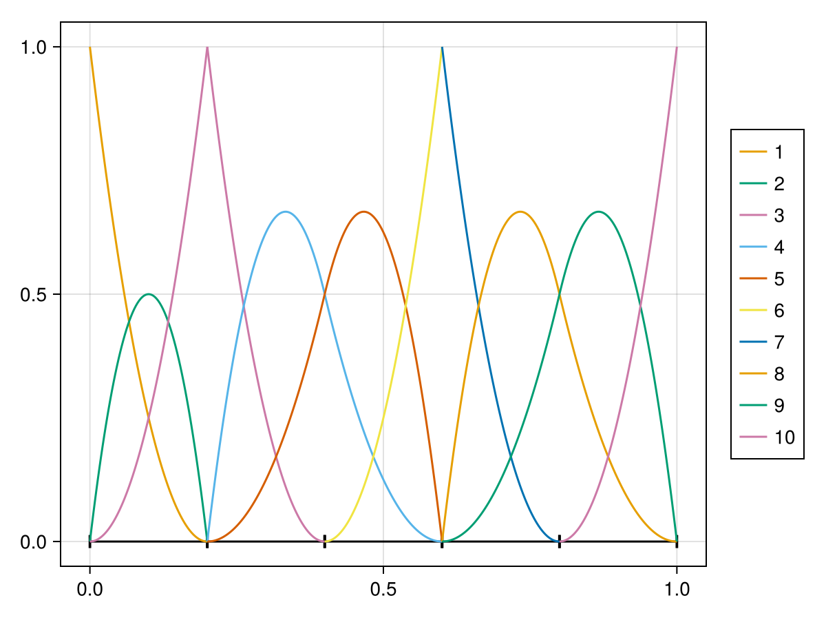-smooth between the first and second elements; -smooth between the second and third elements; -smooth across the third and fourth elements, and so forth. We can confirm this in the next figure:

Now we start by looking at what FunctionSpaces.get_extraction gives us for the first element.

E₁, J₁ = FunctionSpaces.get_extraction(bsp, 1);

E₁ = [1.0 0.0 0.0; 0.0 1.0 0.0; 0.0 0.0 1.0]
J₁ = 1:3

This is telling us the extraction coefficients at the first element are just an identity matrix, and that the permutation is trivial — the bases are in the correct order. This is not a very exciting scenario, so let's look at the third element

E₃, J₃ = FunctionSpaces.get_extraction(bsp, 3)

E₃ = [0.4999999999999999 0.5000000000000001 0.0; 0.0 1.0 0.0; 0.0 0.0 1.0]
J₃ = 1:3

The extraction looks a bit more interesting now, and there are a few things we can do with it:

Changing coefficients

Changing coefficients manually like we are about to do can be quite disastrous, as you will soon see.

We can change the coefficients of so that it is constant across the element.

E₃[:,2] .= 0.5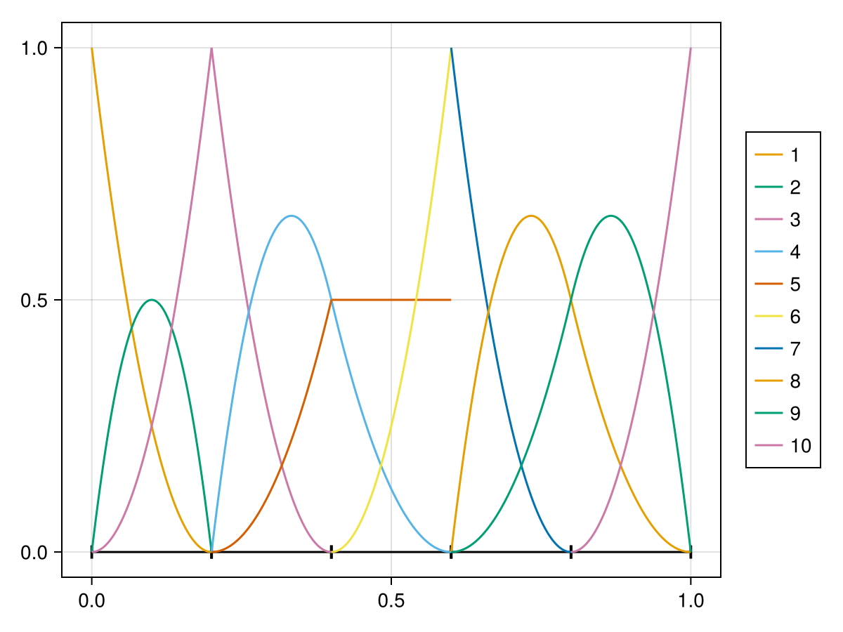

Changing coefficients

Take a moment to notice that changing the coefficients of did two, possibly catastrophic, things:

1. By making constant on the third element, it means we no longer have a local basis for quadratics.

2. The smoothness between the second and third elements also changed from to .

One should always be careful when defining, or changing, extraction coefficients!

Notice that in the changes above we changed the local index of the extraction operator corresponding to a certain global index.

To see what the global indices are at the third element we can call get_basis_indices:

FunctionSpaces.get_basis_indices(bsp, 3)

4:6

We can see that the basis functions supported on this element are the ones labelled [4,5,6]; this is what we expected from the labels in the plots.

Conclusion

As we saw, a framework using extraction coefficients can make defining very complex function spaces efficient, generic and structured. The possibilities are quite vast: you can make any linear combinations you want from a predetermined set of canonical basis functions.