Heat Equation

Background knowledge

A. The Heat Equation in 1D

1. The differential equation

The heat equation in one dimension is given by:

$$\frac{\partial u}{\partial t}-\frac{\partial }{\partial x}\left(\alpha \frac{\partial u}{\partial x}\right)=f\text{for}x\in (0,L)\text{and}t>0$$

where:

• $x$ is the spatial coordinate,

• $t$ is the time,

• $\alpha (x)$ is the spatially-varying thermal diffusivity of the material,

• $u(x,t)$ is the temperature distribution function,

• $f(x,t)$ is a time dependent and spatially varying heat source.

2. Initial and boundary conditions

To solve the heat equation, we must specify initial and boundary conditions: 2. Initial Condition: This refers to the temperature distribution at the initial time $t=0$. We need to know this temperature distribution in our entire domain $(0,L)$.

$$u(x,0)=u_0(x)$$

3. Boundary Conditions: We can specify different types of boundary conditions, i.e., conditions on the boundaries of our domain, $x=0$ and $x=L$.

• Dirichlet Boundary Conditions: This boundary condition means that the temperature is specified at the boundaries of the domain.

  $$u(0,t)=u_0\text{and}u(L,t)=u_L$$

• Neumann Boundary Conditions: This boundary condition means that, instead of the temperature, the derivative of the temperature (which is called the heat flux) is specified at the boundaries of the domain.

  $$\alpha (0)\frac{\partial u}{\partial x}(0,t)=g_0\text{and}\alpha (L)\frac{\partial u}{\partial x}(L,t)=g_L$$

3. Applications

A simplified example where the heat equation can be used is to find out how the temperature is distributed through the outside, insulating walls of your apartment. Look at the image below (source).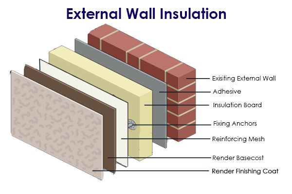

The insulation wall is made up of several materials, each with their own thermal diffusivities ${\alpha }_i(x)$. Imagine that the temperature outside is 0 degrees, and your heating system holds the temperature inside your house at 18 degrees. Then, these are the boundary conditions for the heat equation. Given an initial temperature distribution through the insulation wall, you could use the heat equation to find out how the temperature varies inside the insulation wall.

B. Solving the Heat Equation

1. Disadvantages of the above formulation

Now, if we want to compute the solution of the heat equation as stated above, we run into two difficulties: 2. Lack of exact solutions: For a general function $f$, finding out the exact, analytical solution $u$ is not an easy task. Well, this is not entirely true: finding the solution can be easy enough in one dimension on a domain as simple as $(0,L)$, but in higher dimensions and on more complicated geometries (e.g., imagine the insulation wall of the Guggenheim museum) it is not possible.

3. A restrictive set of solutions: For the above form of the heat equation to make sense, we must also assume that the second-derivatives of the solution $u(x)$ should exist, and that the first derivatives of the thermal diffusivity $\alpha (x)$ should exist. It turns out that this is too strong of a requirement that it not satisfied by many physical systems.

For example, think of the insulation wall - each material in the insulation wall has its own thermal diffusivity which is completely unrelated to the diffusivities of the other materials. As a result, $\alpha (x)$ is a discontinuous function and its first derivatives do not make sense.

2. Tackling the above disadvantages using a discrete & weaker formulation

The above disadvantages are the reason why, in practice, the above strong formulation of the heat equation is not useful. Instead, we formulate a discrete, weak version of the equation which is much more useful in practice. The motivation is: 2. Discrete approximation of unknown exact solutions: Since we don't know the exact solution in general, we try to approximate it. This is the process called discretization. In this process, we fix a finite-dimensional vector space of spatially-varying functions $V_n$ and say that, for any given time $t$, we want to find a function $u_n(\cdot ,t)\in V_n$ which approximates the exact solution $u(\cdot ,t)$. Here, $n$ denotes the dimension of the vector space $V_n$. We expect that as $n\to \mathrm{\infty }$, the solution $u_n(\cdot ,t)\to u(\cdot ,t)$.

3. Weak version of the equation: Since the original equation imposes too strong requirements on the smoothness of $u(x,t)$ and $\alpha (x)$, we instead work with an integral formulation where only the first derivatives of $u(x,t)$ should make sense, and where $\alpha (x)$ is allowed to be discontinuous.

ASSUMPTION: For the sake of simplifying the discussion, from now on we will assume that we are imposing Dirichlet boundary conditions at $x=0$ and $x=L$.

This discrete, weak version of the problem at a fixed time $t$ is stated as: find $u_n(\cdot ,t)\in S_n$ such that

$${\int }_0^L{w}_n\frac{\partial u_n}{\partial t}\mathrm{d}x+{\int }_0^L\alpha \frac{\partial u_n}{\partial x}\frac{\partial w_n}{\partial x}\mathrm{d}x={\int }_0^{L}f{w}_{n}dx,\mathrm{\forall }{w}_n\in W_n,$$

where:

• $S_n:=\{v_n(x)\in V_n:v_n(0)=u_0,v_n(L)=u_L\}$,

• $W_n:=\{v_n(x)\in V_n:v_n(0)=0,v_n(L)=0\}$.

Note the following important things: 2. The above problem tries to find the solution $u_n(\cdot ,t)$ at the fixed time instant $t$.

3. $S_n$ consists of spatially-varying functions in $V_n$ that satisfy the boundary conditions.

4. We want the integral equation above to be satisfied for all functions $w_n\in W_n$, where the function space $W_n$ consists of spatially-varying functions in $V_n$ that satisfy homogeneous (or, equivalently, zero) boundary conditions.

The finite element method

Now we are at a stage where, if we make a choice for $V_n$, we can convert the discrete weak problem into a system of ODEs. This section will explain how.

A. How to choose $V_n$?

1. Choosing $V_n$

In the finite element method, we choose $V_n$ as the space of piecewise-polynomial functions of degree $p$ on a mesh of the domain $(0,L)$.

Meshing the domain

We choose a set of $N+1$ points, $0=x_1<x_1<x_2<\cdots <x_{N+1}=L$, and these points divide the domain $(0,L)$ into smaller subdomains, $(x_i,x_{i+1})$ with $x_i\in (0,L)$, called elements. That is, we assume that there are $N$ elements in our mesh.

ASSUMPTION: In the following code, we will always assume that the mesh is uniform. In other words, $x_{i+1}-x_i$ is equal to $L/N$ for all $i$.

Defining $V_n$

The space $V_n$ is defined as the space of functions $v_n$ such that:

• on any element (i.e., on the interval $(x_i,x_{i+1})$ with $i=1,\dots ,N$) it is a polynomial of degree $p$,

• at each $x_i$, $i=2,\dots ,N$, the function $v_n$ is $C^k$ smooth for some $k\ge 0$.

Once we do this, the vector-space dimension of $V_n$ can be related to the parameters $N,p,k$ as follows:

$$n=(p+1)N-(k+1)(N-1).$$

In other words, there are $n$ basis functions ${\varphi }_i(x)$, $i=1,\dots ,n$, such that any arbitrary $v_n\in V_n$ can be represented as:

$$v_n(x)=\sum _{i=1}^n{c}_i{\varphi }_i(x),$$

for some numbers $c_i\in \mathbb{R}$.

EXAMPLE: $V_n$ with $(N,p,k)=(4,1,0)$.

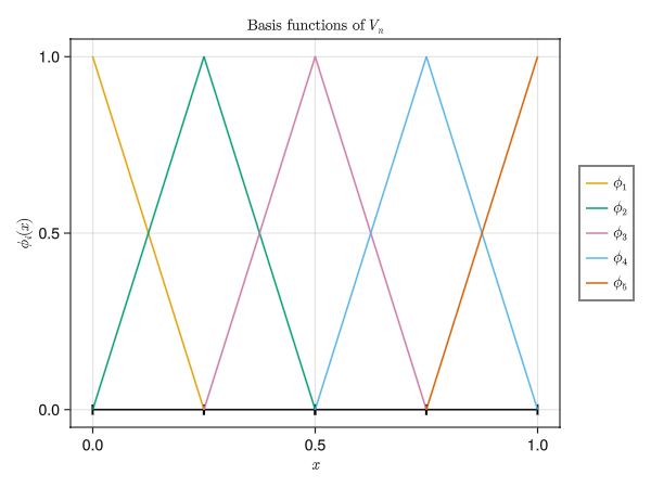
Consider the space of functions that are linear polynomials over each mesh element, and which are $C^0$ smooth (or, equivalently, continuous) at the interfaces $x_i$ between the elements. This space of functions has dimension:

$$n=(p+1)N-(k+1)(N-1)=2\times 4-1\times 3=5.$$

So, we can find 5 basis functions, ${\varphi }_1,{\varphi }_2,\dots {\varphi }_5$, that span the space $V_n$. Run the code below to create such a $V_n$ and look at one such choice of the basis functions called hat functions. Convince yourself that linear combinations of these functions can be used to represent any piecewise-linear polynomial function on the mesh. (Each function is plotted in a different color.)

using Mantis
using GLMakie

# The size of the domain where to solve our problem
L1 = 1.0

# The degree of the piecewise-polynomial basis functions
p1 = 1
# The number of elements in the mesh
N1 = 4
# The smoothness of the basis functions (must be smaller than the polynomial degree, and
# larger than -1)
k1 = 0

# The number of basis functions in the piecewise-polynomial function space
n1 = N1 * (p1 + 1) - (k1 + 1) * (N1 - 1)

# Create the mesh and the function space
breakpoints1 = LinRange(0.0, L1, N1+1)
line_geo1 = Geometry.CartesianGeometry((breakpoints1,))
B1 = FunctionSpaces.BSplineSpace(line_geo1, p1, k1)

fig1 = Mantis.Plot.plot_basis(
    B1;
    label_prefix=L"\phi_",
    title=L"\text{Basis functions of }V_n",
    xlabel=L"x",
    ylabel=L"\phi_i(x)",
)

EXAMPLE: $V_n$ with $(N,p,k)=(4,2,1)$.

Consider now the space of functions that are quadratic polynomials over each mesh element, and which are $C^1$ smooth (or, equivalently, continuous and continuously differentiable) at the interfaces $x_i$ between the elements. This space of functions has dimension:

$$n=(p+1)N-(k+1)(N-1)=3\times 4-2\times 3=6.$$

So, we can find 6 basis functions, ${\varphi }_1,{\varphi }_2,\dots {\varphi }_6$, that span the space $V_n$. Run the code below to create such a $V_n$ and look at one such choice of the basis functions called B-splines. (Each function is plotted in a different color.)

p2 = 2
k2 = 1
n2 = N1 * (p2 + 1) - (k2 + 1) * (N1 - 1)

B2 = FunctionSpaces.BSplineSpace(line_geo1, p2, k2)

fig2 = Mantis.Plot.plot_basis(
    B2;
    label_prefix=L"\phi_",
    title=L"\text{Basis functions of }V_n",
    xlabel=L"x",
    ylabel=L"\phi_i(x)",
)

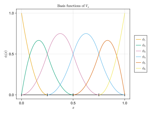
Note: In both of the above examples, the only functions non-zero at $x=0$ and $x=L$ are ${\varphi }_1$ and ${\varphi }_n$. This means that, in particular, the functions ${\varphi }_2,\dots ,{\varphi }_{n-1}$ form a basis for $W_n$. We will use this fact later on.

Since, at each time instant $t$, our approximate solution $u_n(x,t)$ is represented as a linear combination of the basis functions ${\varphi }_i$, $i=1,\dots ,n$, that span $V_n$, this means that our approximate solution has the following form:

$$u_n(x,t)=\sum _{i=1}^n{c}_i(t){\varphi }_i(x).$$

In other words, the coefficients of the linear combination are time-dependent. But we can say more! Since $u_n(0,t)=u_0$ and $u_n(L,t)=u_L$ are the boundary conditions, then we must have:

$$u_n(x,t)=u_0{\varphi }_1(x)+\sum _{i=2}^{n-1}{c}_i(t){\varphi }_i(x)+u_L{\varphi }_n(x).$$

That is, the only unknown coefficients in the above expression are $c_i(t)$, $i=2,\dots ,n-1$.

ASSUMPTION: For simplicity, we assume that $u_0$ and $u_L$ are constants.

B. Assembling the System of ODEs

Now that we have arrived at an explicit form of our approximate solution to the weak problem, let us see how the discrete weak problem leads to a system of ODEs for the coefficients $c_i(t)$. This process is called assembly and it leads to a system of ODEs that looks like:

$$\mathbf{M}\frac{d\mathbf{C}}{dt}+\mathbf{K}\mathbf{C}=\mathbf{F}-u_0{\mathbf{F}}^{b,0}-u_L{\mathbf{F}}^{b,L},$$

where we have arranged the unknown coefficients $c_i(t)$ in a vector $\mathbf{C}(t):=[c_2(t),c_3(t),\dots ,c_{n-1}(t)]$.

Some terminology: in the above system of ODEs, $\mathbf{M}$ is called the mass matrix, $\mathbf{K}$ is called the stiffness matrix, $\mathbf{F}$ is called the load vector, ${\mathbf{F}}^{b,0}$ and ${\mathbf{F}}^{b,L}$ are the contributions of the known coefficients ($c_1$ and $c_n$) to the loading, respectively, and $\mathbf{C}$ is the vector of unknown coefficients that define the solution.

The idea behind assembly is simple. We substitute the assumed form of our discrete solution $u_n$ into the discrete weak problem. This gives us:

$${\int }_0^L{w}_n\frac{\partial }{\partial t}(\sum _{j=1}^n{c}_j{\varphi }_j)\mathrm{d}x+{\int }_0^L\alpha \frac{\partial w_n}{\partial x}\frac{\partial }{\partial x}(\sum _{j=1}^n{c}_j{\varphi }_j)\mathrm{d}x={\int }_0^{L}f{w}_{n}dx,\mathrm{\forall }{w}_n\in W_n,$$

Since we need to satisfy the above equation for all $w_n\in W_n$, and since the above equation is linear in $w_n$, it is actually enough if we satisfy the above equation for the basis functions that span $W_n$, i.e., ${\varphi }_i$, $i=2,\dots ,n-1$. Then, choosing $w_n={\varphi }_i$ gives us the following equation, and we get one such equation for each $i=2,\dots ,n-1$,

$${\int }_0^L{\varphi }_i\frac{\partial }{\partial t}(\sum _{j=1}^n{c}_j{\varphi }_j)\mathrm{d}x+{\int }_0^L\alpha \frac{\partial {\varphi }_i}{\partial x}\frac{\partial }{\partial x}(\sum _{j=1}^n{c}_j{\varphi }_j)\mathrm{d}x={\int }_0^{L}f{\varphi }_{i}dx.$$

We can rearrange this equation as:

$$\sum _{j=2}^{n-1}\frac{d{c}_j}{dt}{\int }_0^L{\varphi }_i{\varphi }_j\mathrm{d}x+\sum _{j=2}^{n-1}{c}_j{\int }_0^L\alpha \frac{d{\varphi }_i}{dx}\frac{d{\varphi }_j}{dx}\mathrm{d}x={\int }_0^{L}f{\varphi }_i-u_0{\int }_0^L\alpha \frac{d{\varphi }_i}{dx}\frac{d{\varphi }_1}{dx}dx-u_L{\int }_0^L\alpha \frac{d{\varphi }_i}{dx}\frac{d{\varphi }_n}{dx}dx.$$

Then, it is easy to see that this equation represents the ODE system at the beginning of this section by defining:

• ${\mathbf{M}}_{ij}={\int }_0^L{\varphi }_i{\varphi }_j\mathrm{d}x$,

• ${\mathbf{K}}_{ij}={\int }_0^L\frac{d{\varphi }_i}{dx}\frac{d{\varphi }_j}{dx}\mathrm{d}x$,

• ${\mathbf{F}}_i={\int }_0^L{\varphi }_{i}f\mathrm{d}x$,

• ${\mathbf{F}}_i^{b,0}={\int }_0^L\alpha \frac{d{\varphi }_i}{dx}\frac{d{\varphi }_1}{dx}dx$,

• ${\mathbf{F}}_i^{b,L}={\int }_0^L\alpha \frac{d{\varphi }_i}{dx}\frac{d{\varphi }_n}{dx}dx.$

To assemble the matrices $\mathsf{M}$ and $\mathsf{K}$ and the vectors $F$, $F^{b,0}$ and $F^{b,L}$, we first must define $\alpha$ and $f$.

Before choosing our forcing term, it is relevant to briefly analyse the behavior of our solution. We saw that our weak form of the equation is

$${\int }_0^L{w}_n\frac{\partial u_n}{\partial t}\mathrm{d}x+{\int }_0^L\alpha \frac{\partial u_n}{\partial x}\frac{\partial w_n}{\partial x}\mathrm{d}x={\int }_0^{L}f{w}_{n}dx,\mathrm{\forall }{w}_n\in W_n,$$

Since we have Dirichlet boundary conditions (i.e., we enforce the value of the temperature on both sides of our interval), if we prescribe a stationary heat source, the solution will evolve to a stationary state. This stationary state, $u_h^s$ will be the one that satisfies

$${\int }_0^L\alpha \frac{\partial u_n}{\partial x}\frac{\partial w_n}{\partial x}\mathrm{d}x={\int }_0^{L}f{w}_{n}dx,\mathrm{\forall }{w}_n\in W_n,$$

or in matrix form

$$\mathbf{K}\mathbf{C}=\mathbf{F}-u_0{\mathbf{F}}^{b,0}-u_L{\mathbf{F}}^{b,L}.$$

Additionally, if $\alpha$ is constant, and if the heat source $f$ is smooth, then we can easily construct analytical solutions to the stationary state. For example,

$$u^s(x,t)=1+\frac{1}{2}\cos \left(\frac{2\pi }{L}x\right),$$

if the heat source is

$$f(x,t)=\frac{2\alpha {\pi }^2}{L^2}\cos \left(\frac{2\pi }{L}x\right).$$

We choose a finite element space with $(N,p,k)=(10,2,1)$, i.e., with more elements compared to the last example. This is to ensure that we have sufficient accuracy for computing a decent solution.

# The size of the domain where to solve our problem
L = 1.0
# The number of elements in the mesh
num_elements = 10
line_geometry = Geometry.create_cartesian_box((0.0,), (L,), (num_elements,))

# The degree of the piecewise-polynomial basis functions
polynomial_degree = 2
# The smoothness of the basis functions (-1 <= smoothness <= p-1)
smoothness = 1

# The piecewise-polynomial function space
V = FunctionSpaces.BSplineSpace(line_geometry, polynomial_degree, smoothness)
# The number of basis functions in the piecewise-polynomial function space
num_basis_functions = FunctionSpaces.get_num_basis(V)

# Use this function space as a differential form
V⁰ = Forms.FormSpace(0, V, L"V^0")

# Thermal diffusivity
const alpha = 1.0

# Analytical solution
u_analytical_expression(x) = [1.0 .+ 0.5*cos.((2.0*π/L)*x[:, 1])]
u_analytical = Mantis.Forms.AnalyticalFormField(
    0, u_analytical_expression, line_geometry, L"u_{\text{exact}}"
)

# Right hand side
f_expression(x) = [@. alpha*0.5*(4.0*(π^2)/(L^2))*cos(2.0*π*x[:, 1]/L)]
f = Mantis.Forms.AnalyticalFormField(0, f_expression, line_geometry, "f")

function assemble_system_matrices(
    V::Forms.FormSpace,
    f::Forms.AnalyticalFormField,
    alpha::Float64,
    dΩ::Quadrature.AbstractQuadratureRule,
)
    # assemble L2 inner-product matrix
    weak_form_inputs = Assemblers.WeakFormInputs(V, f)
    lhs_expressions, rhs_expressions = Assemblers.L2_projection(weak_form_inputs, dΩ)
    weak_form = Assemblers.WeakForm(lhs_expressions, rhs_expressions, weak_form_inputs)
    M, _ = Assemblers.assemble(weak_form)

    # assemble H1 inner-product matrix
    weak_form_inputs = Assemblers.WeakFormInputs(V, f)
    lhs_expressions, rhs_expressions = Assemblers.zero_form_hodge_laplacian(
        weak_form_inputs, dΩ
    )
    weak_form = Assemblers.WeakForm(lhs_expressions, rhs_expressions, weak_form_inputs)
    # bc = Forms.set_dirichlet_boundary_conditions(V, 0.0)
    K, f = Assemblers.assemble(weak_form)

    return M, alpha .* K, f
end

# Define the quadrature
quadrature_degree = polynomial_degree + 2
∫ = Quadrature.gauss_legendre(quadrature_degree)
dΩ = Quadrature.StandardQuadrature(∫, num_elements)

# Assemble the matrices
M, K, F = assemble_system_matrices(V⁰, f, alpha, dΩ)

# Remove the unecessary parts of the matrices
F = Vector(F[2:(end - 1)])

K_0 = Vector(K[2:(end - 1), 1])
K_L = Vector(K[2:(end - 1), end])

M = M[2:(end - 1), 2:(end - 1)]
K = K[2:(end - 1), 2:(end - 1)]

# Boundary conditions
u_0 = 1.5
u_L = 1.5

# Solution field
u_h = Mantis.Forms.FormField(V⁰, zeros(Forms.get_num_basis(V⁰)), "u_h")

# With boundary values set
u_h.coefficients[1] = u_0
u_h.coefficients[end] = u_L

# Solve for the unknown coefficients
u_h.coefficients[2:(end - 1)] = K \ (F - u_0*K_0 - u_L*K_L)

# Plot the error with respect to the analytical solution
error = u_analytical - u_h

# Compute the error norm
error_nom = Analysis.L2_norm(error, dΩ)

0.0005600033681980221

Time Integration

We will now consider a specific time integrator to evolve our solution in time: the midpoint rule.

The midpoint rule is the lowest order Gauss integrator and, for linear systems (as is our case), is an explicit integrator. Additionally, it can be interpreted as a Runge-Kutta method (i.e., it has an associated Butcher tableau). Given a first order ODE in the time interval $(0,T)$

$$\frac{\mathrm{d}g}{\mathrm{d}t}=f(t,g(t))$$

with initial condition $g(0)=g_0$, the midpoint rule to evolve the solution from the time instant $t_k$ to the time instant $t_{k+1}=t_k+\mathrm{\Delta }t$ is

$$g_{k+1}=g_k+\mathrm{\Delta }tf(t+\frac{\mathrm{\Delta }t}{2},\frac{g_{k+1}+g_k}{2}).$$

where $g_k=g(k\mathrm{\Delta }t)$.

The spatial discretisation process has left us with the following system of ODEs:

$$\mathbf{M}\frac{d\mathbf{C}}{dt}=-\mathbf{K}\mathbf{C}+\mathbf{F}-u_0{\mathbf{F}}^{b,0}-u_L{\mathbf{F}}^{b,L}.$$

We can integrate this in time using the pre-implemented midpoint rule.

Explicit ODE with a matrix solve

While the integrator is considered explicit, this only holds for simple ODEs. In our case, we have a coupled system of ODEs, so that we do have to use a matrix solver.

# Time step size and final time.
const dt = 0.001
const num_time_steps = 501

# Here, we encode the ODE information for the time integrator. We are using LinearSolve's
# ability to cache the factorised M matrix. Since this matrix does not change per
# timestep, we can reuse the factorisation. This is more efficient than refactorising every
# step.
import LinearSolve as LS
const prob = LS.LinearProblem(M, zeros(Forms.get_num_basis(V⁰)-2))
const linsolve = LS.init(prob)
function heat_equation_solver(output, C::Vector{Float64}, t::Float64)
    linsolve.b = (-K * C + F - u_0 * K_0 - u_L * K_L)
    output .= LS.solve!(linsolve)
    return output
end
const heat_equation = TimeIntegrators.define_explicit_ode(heat_equation_solver)

scheme = TimeIntegrators.EXPLICIT_MIDPOINT

# We also create a helper function to easily evaluate our solution.
function evaluate_solution(u_h)
    geometry = Forms.get_geometry(u_h)
    num_elements = Geometry.get_num_elements(geometry)
    xi = Points.CartesianPoints((LinRange(0.0, 1.0, 25),))
    all_x = Vector{Float64}(undef, 25 * num_elements)
    all_values = Vector{Float64}(undef, 25 * num_elements)
    for element_id in 1:num_elements
        form_eval, _ = Forms.evaluate(u_h, element_id, xi)
        x = Geometry.evaluate(geometry, element_id, xi)

        all_x[((element_id - 1) * 25 + 1):((element_id) * 25)] = x[:]
        all_values[((element_id - 1) * 25 + 1):((element_id) * 25)] = form_eval[1]
    end

    return all_x, all_values
end

# We project the initial condition onto our form space
u_initial_expression(x) = [@. 1.5 + sin((2.0*π/L)*x[:, 1])]
u_initial = Forms.AnalyticalFormField(0, u_initial_expression, line_geometry, "u")
u_hi = Assemblers.solve_L2_projection(V⁰, u_initial, dΩ)

# Enforce the boundary condition on the initial condition, just in case the initial
# condition does not satisfy the boundary conditions already
u_hi.coefficients[1] = u_0
u_hi.coefficients[end] = u_L

# Initialise the time scheme
const u_h_n = TimeIntegrators.initialise_scheme(u_hi.coefficients[2:(end - 1)], scheme)

Mantis.TimeIntegrators.TimeIntegrationSolution{Mantis.TimeIntegrators.Explicit{2, 1, Float64, 4, 2, 1}, Nothing, Float64, Nothing}(10, [1.825836023728004; 2.3496538725133327; … ; 0.6503461274866671; 1.1741639762719966;;], Mantis.TimeIntegrators.Explicit{2, 1, Float64, 4, 2, 1}([0.0 0.0; 0.5 0.0], [0.0 1.0], [1.0; 1.0;;], [1.0;;], [0.0, 0.5], Mantis.TimeIntegrators.TimeLevels([0], Int64[], Int64[]), 2), nothing, 0, [6.9290475962142e-310; 6.929085453905e-310; … ; 6.9290459367165e-310; 6.92904593671806e-310;;], [0.0 0.0; 0.0 0.0; … ; 0.0 0.0; 0.0 0.0], [0.0 0.0; 0.0 0.0; … ; 0.0 0.0; 0.0 0.0], nothing, [0.0, 0.0, 0.0, 0.0, 0.0, 0.0, 0.0, 0.0, 0.0, 0.0], [0.0, 0.0, 0.0, 0.0, 0.0, 0.0, 0.0, 0.0, 0.0, 0.0])

Now we are set to march our equation in time. We will also create a video, which is why we set up the time Observable. The all_y variable is a lift, which is Makie's way of expressing a dependency. That is, as soon as we update time, Makie will automatically update all other variables in the plot that depend on time. In our case, this is the all_y variable, which calls TimeIntegrators.time_integrate! to advance our solution.

# We use Printf to print the time in our animation.
using Printf

time = Observable(dt)

all_y = lift(time) do t
    TimeIntegrators.time_integrate!(u_h_n, heat_equation, t, dt)

    u_hi.coefficients[2:(end - 1)] = TimeIntegrators.get_solution(u_h_n)

    all_x, all_values = evaluate_solution(u_hi)

    return all_values
end

all_x, all_values = evaluate_solution(u_hi)
fig = lines(
    all_x,
    all_y;
    color=:blue,
    axis=(
        title=@lift("t = $(@sprintf("%0.2f", round($time, digits = 2)))"),
        limits=(0.0, 1.0, 0.0, 3.0),
    ),
)

xe, ye = evaluate_solution(u_analytical)
lines!(xe, ye; color=:black, label="exact")

record(
    fig,
    "heat_equation_1d.mp4",
    LinRange(dt, dt*num_time_steps, num_time_steps);
    framerate=30,
) do t
    return time[] = t
end

"heat_equation_1d.mp4"

---

This page was generated using Literate.jl.