One-dimensional mapped geometry

This example will guide through the process of defining a one-dimensional mapped geometry in Mantis.jl.

Background

A mapped geometry has two essential ingredients: an original geometry and a mapping. For our purposes, we can consider the original geometry as a Cartesian geometry — although this might not be the case.

Associated with each element $e_i$ of a Cartesian geometry is an implicit map ${\phi }_i$, which is unrelated to the mapping of the mapped geometry. Each ${\phi }_i$ has the purpose of defining how to go from a point $\xi$ on the canonical element $[0,1]$ to a point $\hat{\xi }$ on $e_i$. In the case of a Cartesian geometry, if we define by $e_{i,1}$ and $e_{i,2}$ the endpoints of the element $e_i$, we have

$$\hat{\xi }={\phi }_i(\xi )=e_{i,1}+\xi (e_{i,2}-e_{i,1}).$$

This is the reason most of the evaluate methods throughout Mantis.jl take as part of their inputs an element_id and a set of points; the first tells us which ${\phi }_i$ to consider, and the second which points of the canonical element are relevant.

With this in mind, we can move to the second ingredient: the mapping. This will be some user-provided function $\varphi$ that will be applied to $\hat{\xi }$, essentially transforming our original Cartesian geometry. This means a point $x$ in the mapped geometry is defined as

$$x=\varphi (\hat{\xi })=\varphi ({\phi }_i(\xi )),$$

where ${\phi }_i$ is chosen depending on which element $\hat{\xi }$ lies in.

It is important to keep these relationships in mind since the derivatives are computed with respect to the canonical coordinate $\xi$.

$$\frac{d\varphi }{d\xi }=\frac{d\varphi }{d\hat{\xi }}\frac{d\hat{\xi }}{d\xi }=\frac{d\varphi }{d\hat{\xi }}(e_{i,2}-e_{i,1}),$$

and

$$\frac{d^2\varphi }{d{\xi }^2}=\frac{d^2\varphi }{d{\hat{\xi }}^2}{\left(\frac{d\hat{\xi }}{d\xi }\right)}^2+\frac{d\varphi }{d\hat{\xi }}\frac{d^2\hat{\xi }}{d{\xi }^2}=\frac{d^2\varphi }{d{\hat{\xi }}^2}(e_{i,2}-e_{i,1}{)}^2,$$

with the second term in the middle expression being zero for a Cartesian geometry.

Implementation

using Mantis

First we will set-up the original geometry.

starting_point = (1.0,)
box_size = (3.0,)
num_elements = (3,)
original_geo = Geometry.create_cartesian_box(starting_point, box_size, num_elements)

Mantis.Geometry.CartesianGeometry{1, 1, 1, Tuple{Tuple{LinRange{Float64, Int64}}}, Tuple{CartesianIndices{1, Tuple{Base.OneTo{Int64}}}}, Tuple{LinearIndices{1, Tuple{Base.OneTo{Int64}}}}}(((LinRange{Float64}(1.0, 4.0, 4),),), (CartesianIndices((3,)),), (LinearIndices((Base.OneTo(3),)),))

For a quick sanity check, we can evaluate the endpoints of our 1D geometry. These should be equal to starting_point and starting_point + box_size, respectively.

fp, lp = starting_point[1], (starting_point[1] + box_size[1]) # First and last point.
fe, le = 1, num_elements[1] # First and last element.
Geometry.evaluate(original_geo, 1, Points.PointSet(([0.0],)))[1] == fp
Geometry.evaluate(original_geo, le, Points.PointSet(([1.0],)))[1] == lp

true

We can take a look at the first and second derivatives, to see if they are what we expect. To understand the output types of jacobian and hessian we refer the reader to Mantis.Geometry.jacobian and Mantis.Geometry.hessian.

dφᵢ = box_size[1] / le
Geometry.jacobian(original_geo, 1, Points.PointSet(([0.0],)))[1][1] == dφᵢ
Geometry.jacobian(original_geo, 3, Points.PointSet(([1.0],)))[1][1] == dφᵢ
Geometry.hessian(original_geo, 1, Points.PointSet(([0.0],)))[1][1][1] == 0.0
Geometry.hessian(original_geo, 3, Points.PointSet(([1.0],)))[1][1][1] == 0.0

true

We have the first ingredient needed to build a MappedGeometry; now we just need to define what our mapping $\varphi$ is, using the structure Geometry.Mapping. This structure will contain the definition of $\varphi$, $\frac{d\varphi }{d\hat{\xi }}$ and, optionally, $\frac{d^2\varphi }{d{\hat{\xi }}^2}$. Because we will choose a simple mapping we can provide both the first and second derivatives. (The argument (1, 1) in the function call just means that both our original and mapped geometries can be represented in just 1 dimension.)

exponent = 3
ϕ_map(ξ̂) = ξ̂^exponent
dϕ_map(ξ̂) = exponent * ξ̂^(exponent - 1)
d2ϕ_map(ξ̂) = exponent * (exponent - 1) * ξ̂^(exponent - 2)
ϕ = Geometry.Mapping(
    (1, 1), ξ̂ -> ϕ_map.(ξ̂[:, 1]), ξ̂ -> dϕ_map.(ξ̂[:, 1]), ξ̂ -> d2ϕ_map.(ξ̂[:, 1])
)

Mantis.Geometry.Mapping{1, 1, Main.var"Main".var"#4#5", Main.var"Main".var"#6#7", Main.var"Main".var"#8#9"}(Main.var"Main".var"#4#5"(), Main.var"Main".var"#6#7"(), Main.var"Main".var"#8#9"())

We can now put both pieces together and define our mapped geometry.

geo = Geometry.MappedGeometry(original_geo, ϕ)

Mantis.Geometry.MappedGeometry{1, 1, 1, Mantis.Geometry.CartesianGeometry{1, 1, 1, Tuple{Tuple{LinRange{Float64, Int64}}}, Tuple{CartesianIndices{1, Tuple{Base.OneTo{Int64}}}}, Tuple{LinearIndices{1, Tuple{Base.OneTo{Int64}}}}}, Mantis.Geometry.Mapping{1, 1, Main.var"Main".var"#4#5", Main.var"Main".var"#6#7", Main.var"Main".var"#8#9"}}(Mantis.Geometry.CartesianGeometry{1, 1, 1, Tuple{Tuple{LinRange{Float64, Int64}}}, Tuple{CartesianIndices{1, Tuple{Base.OneTo{Int64}}}}, Tuple{LinearIndices{1, Tuple{Base.OneTo{Int64}}}}}(((LinRange{Float64}(1.0, 4.0, 4),),), (CartesianIndices((3,)),), (LinearIndices((Base.OneTo(3),)),)), Mantis.Geometry.Mapping{1, 1, Main.var"Main".var"#4#5", Main.var"Main".var"#6#7", Main.var"Main".var"#8#9"}(Main.var"Main".var"#4#5"(), Main.var"Main".var"#6#7"(), Main.var"Main".var"#8#9"()), 3, (3,))

We can repeat the sanity check we previously did, where we now expect that evaluating the endpoints gives us ϕ(starting_point) and ϕ(starting_point + box_size), and the derivatives are as in Background.

Geometry.evaluate(geo, 1, Points.PointSet(([0.0],)))[1] == ϕ_map(fp)
Geometry.evaluate(geo, le, Points.PointSet(([1.0],)))[1] == ϕ_map(lp)
Geometry.jacobian(geo, 1, Points.PointSet(([0.0],)))[1][1] == dϕ_map(fp) * dφᵢ
Geometry.jacobian(geo, le, Points.PointSet(([1.0],)))[1][1] == dϕ_map(lp) * dφᵢ
Geometry.hessian(geo, 1, Points.PointSet(([0.0],)))[1][1][1] == d2ϕ_map(fp) * dφᵢ^2
Geometry.hessian(geo, le, Points.PointSet(([1.0],)))[1][1][1] == d2ϕ_map(lp) * dφᵢ^2

true

Finally, we will take a look at both geometries to have a visual confirmation of our intiutions.

using GLMakie

el_endpoints = Points.PointSet(([0.0, 1.0],))
zrs = zeros(2)

2-element Vector{Float64}:
 0.0
 0.0

Plot of the Cartesian geometry

fig = Figure()
og_ax = Axis(
    fig[1, 1];
    title="Cartesian geometry",
    xlabel="x",
    ylabel="",
    xticks=LinRange(fp, lp, le + 1),
    limits=((fp - 0.1, lp + 0.1), (-0.5, 0.5)),
)
for element in 1:le
    xs = Geometry.evaluate(original_geo, element, el_endpoints)
    lines!(og_ax, xs[:, 1], zrs; linewidth=3)
    scatter!(og_ax, xs[:, 1], zrs; color=:black, markersize=10)
end

Plot of the mapped geometry

xticks_mapped = [ϕ_map(p) for p in LinRange(fp, lp, le + 1)]
mp_ax = Axis(
    fig[2, 1];
    title="Mapped geometry",
    xlabel="x",
    xticks=xticks_mapped,
    limits=((ϕ_map(fp) - 1, ϕ_map(lp) + 1), (-0.5, 0.5)),
)
for element in 1:le
    xs = Geometry.evaluate(geo, element, el_endpoints)
    lines!(mp_ax, xs[:, 1], zrs; linewidth=3)
    scatter!(mp_ax, xs[:, 1], zrs; color=:black, markersize=10)
end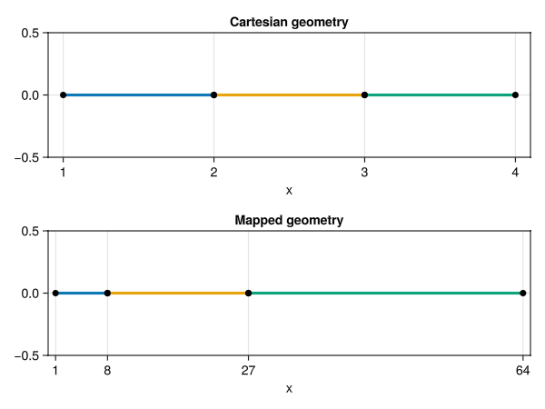

---

This page was generated using Literate.jl.